VIRGO SPM dataset
[1]:
import os

import numpy as np
import pandas as pd
import pywt

from tsipy.correction import compute_exposure, correct_degradation, load_model
from tsipy.utils import (
    plot_signals,
    plot_signals_history,
    pprint,
    pprint_block,
)
Load corrected dataset by C. Fröhlich
[2]:
import datetime

def load_dat_file(file_name : str, directory, n_cols : int, sep="  ") -> pd.DataFrame:
    rows = []
    with open(os.path.join(directory, file_name), "r") as f:
        line = f.readline()
        n_header = int(line.strip().split(";")[0].strip())

        i = 1
        while True:
            line = f.readline()
            i += 1

            # Skip header
            if i <= n_header:
                continue

            # EOF with empty line
            if not line:
                break

            line = line.strip().split(sep)

            if len(line) != n_cols:
                raise ValueError(f"Invalid number of columns {len(line)} in line {i}.")

            rows.append(line)

    data = np.array(rows)
    return data

def parse_timestamp(timestamp, start_date):
    date_str, day_frac = timestamp.split(".")

    date = datetime.datetime.strptime(date_str, "%Y-%m-%d")
    time_delta = date - start_date
    return time_delta.days + float(f"0.{day_frac}")

def load_data_spm(file_name : str, directory="../data") -> pd.DataFrame:
    if f"{file_name}.h5" in os.listdir(directory):
        return pd.read_hdf(os.path.join(directory, f"{file_name}.h5"), "table")

    if file_name == "spm_level2_claus":
        data = load_dat_file("spm_level2_claus.dat", "../data", 4)
        data = pd.DataFrame(data, columns=["t", "r", "g", "b"])
        data["t"] = data["t"].map(lambda x: parse_timestamp(x, datetime.datetime(1996, 4, 17)))
        for channel in ["r", "g", "b"]:
            channel_data = np.copy(data[channel].values.astype(float))
            nan_ids = np.equal(channel_data, -9.99999)
            channel_data[nan_ids] = np.nan
            data[channel] = channel_data

        data.to_hdf(os.path.join(directory, f"{file_name}.h5"), "table", mode="w")
        return data
[3]:
data = load_data_spm("spm_level2_claus")
t = data["t"].values
r = data["r"].values
g = data["g"].values
b = data["b"].values
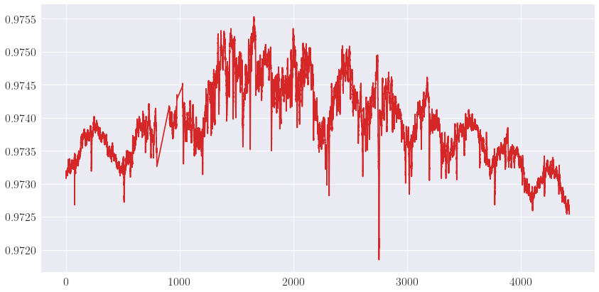
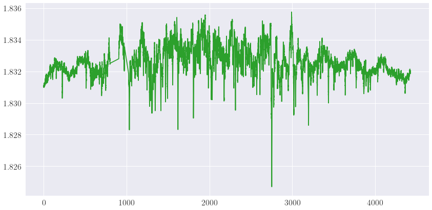
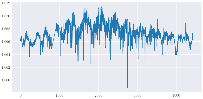
_ = plot_signals([(t, r, "$r$", {"c": "tab:red"})])
_ = plot_signals([(t, g, "$g$", {"c": "tab:green"})])
_ = plot_signals([(t, b, "$b$", {"c": "tab:blue"})])
Load level-1 data
[4]:
def load_data_spm(file_name : str, directory="../data", n_cols=3) -> pd.DataFrame:
    if f"{file_name}.h5" in os.listdir(directory):
        return pd.read_hdf(os.path.join(directory, f"{file_name}.h5"), "table")

    rows = []
    with open(os.path.join(directory, f"{file_name}.txt"), "r") as f:
        i = 0
        while True:
            line = f.readline()
            line = line.strip().split()

            i += 1
            # EOF with empty line
            if not line:
                break

            if len(line) != n_cols:
                print(i, line)
                raise ValueError("Line {} does not have 3 entries: {}".format(i, line))

            rows.append(line)

    data = np.array(rows).astype(np.float)
    data = pd.DataFrame(data, columns=["t", "a", "b"])

    data.to_hdf(os.path.join(directory, f"{file_name}.h5"), "table", mode="w")
    return data
[43]:
def moving_filter(x : np.ndarray, n_window : int = 11, n_std : int = 2):
    x = pd.Series(x)
    x_mean = x.rolling(n_window, min_periods=1, center=True).mean()
    x_std = x.rolling(n_window, min_periods=1, center=True).std()

    nan_ids = np.greater(np.abs(x - x_mean),  n_std * x_std)
    print(np.sum(nan_ids), nan_ids.size)
    return nan_ids
[60]:
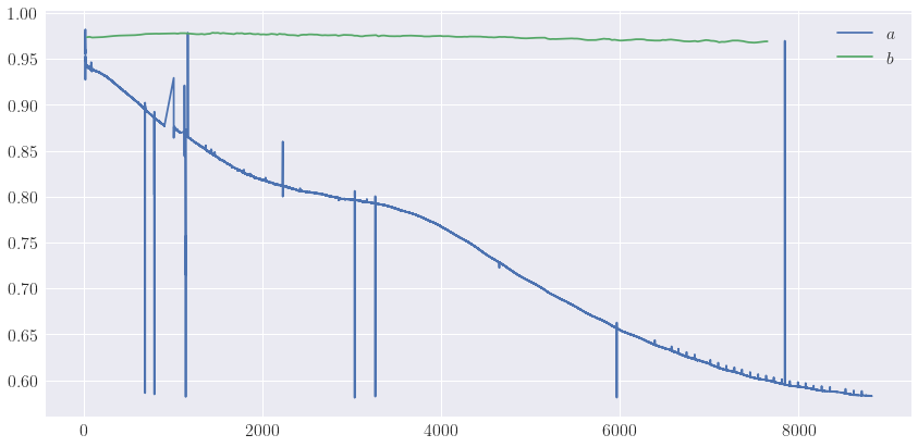
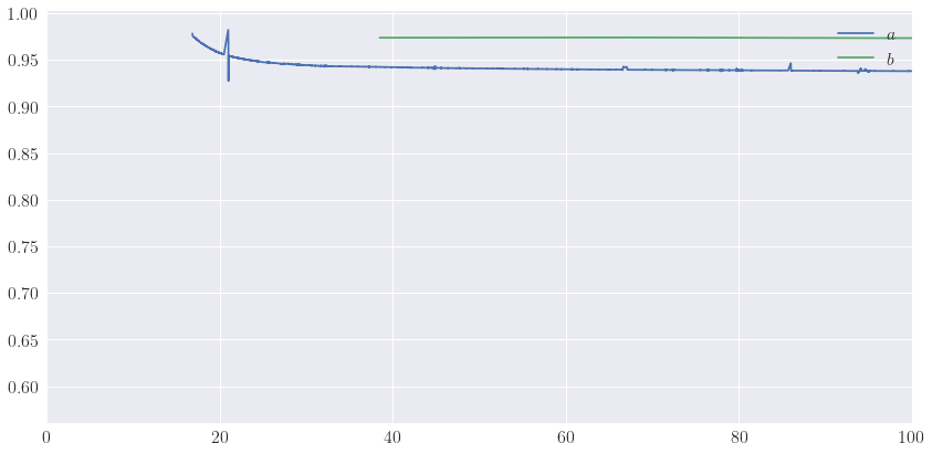
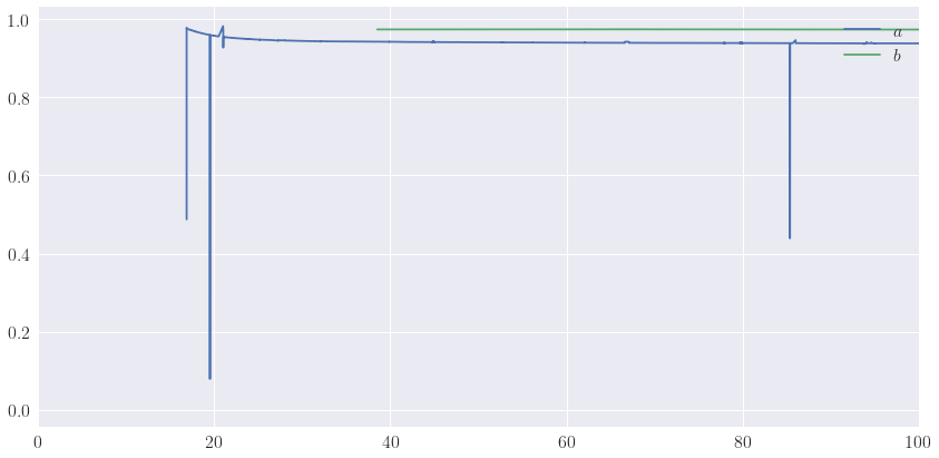
data = load_data_spm(file_name="spm_red_level1", directory="../data", n_cols=3)

t = data["t"].values
a = data["a"].values
b = data["b"].values

a_out = np.copy(a)

nan_ids = np.less(a, 0.58)
a[nan_ids] = np.nan

nan_ids = np.logical_or(nan_ids, moving_filter(a, n_window=200, n_std=5))
a[nan_ids] = np.nan
a_out[~nan_ids] = np.nan

fig, ax = plot_signals(
    [(t, a, "$a$", {}), (t, b, "$b$", {})], legend="upper right"
)
# ax.scatter(t, a_out, label="$a_o$", c="tab:red")

_ = plot_signals(
    [(t, a, "$a$", {}), (t, b, "$b$", {})], legend="upper right", x_lim=(0.0, 100.0)
)
552 12434400
[6]:
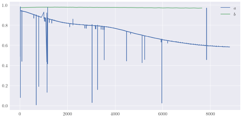
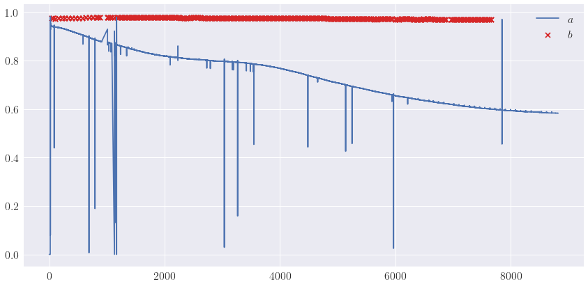
data = load_data_spm(file_name="spm_red_detrended", directory="../data", n_cols=3)

t = data["t"].values
a = data["a"].values
b = data["b"].values

data["a"][data["a"] < 0.005] = np.nan

_ = plot_signals(
    [(t, a, "$a$", {}), (t, b, "$b$", {})], legend="upper right"
)

_ = plot_signals(
    [(t, a, "$a$", {}), (t, b, "$b$", {})], legend="upper right", x_lim=(0.0, 100.0)
)
[ ]:
[3]:
pprint_block("SPM Dataset", level=1)
data = load_data_spm("SpmRed", directory="../data")

# Treat zero-measurements as nans
data["a"][data["a"] == 0.0] = np.nan

# Compute exposure
e_a = compute_exposure(data["a"].values)
e_b = compute_exposure(data["b"].values)
max_e = max(np.max(e_a), np.max(e_b))
e_a /= max_e
e_b /= max_e
data["e_a"] = e_a
data["e_b"] = e_b

# Channel measurements
data_a = data[["t", "a", "e_a"]].dropna()
data_b = data[["t", "b", "e_b"]].dropna()

t_a_nn, t_b_nn = data_a["t"].values, data_b["t"].values
a_nn, b_nn = data_a["a"].values, data_b["b"].values
e_a_nn, e_b_nn = data_a["e_a"].values, data_b["e_b"].values

pprint("Signal", level=0)
pprint("- t_a_nn", t_a_nn.shape, level=1)
pprint("- a_nn", a_nn.shape, level=1)
pprint("- e_a_nn", e_a_nn.shape, level=1)

pprint("Signal", level=0)
pprint("- t_b_nn", t_b_nn.shape, level=1)
pprint("- b_nn", b_nn.shape, level=1)
pprint("- e_b_nn", e_b_nn.shape, level=1)

# Mutual measurements
pprint_block("Simultaneous measurements", level=1)
data_m = data[["t", "a", "b", "e_a", "e_b"]].dropna()
t_m = data_m["t"].values
a_m, b_m = data_m["a"].values, data_m["b"].values
e_a_m, e_b_m = data_m["e_a"].values, data_m["e_b"].values

pprint("Signal", level=0)
pprint("- t_m", t_m.shape, level=1)
pprint("- a_m", a_m.shape, level=1)
pprint("- e_a_m", e_a_m.shape, level=1)

pprint("Signal", level=0)
pprint("- t_m", t_m.shape, level=1)
pprint("- b_m", b_m.shape, level=1)
pprint("- e_b_m", e_b_m.shape, level=1)
    SPM Dataset
---------------------------------------------------------------------------
Signal
    - t_a_nn                                      (12385572,)
    - a_nn                                        (12385572,)
    - e_a_nn                                      (12385572,)
Signal
    - t_b_nn                                      (711,)
    - b_nn                                        (711,)
    - e_b_nn                                      (711,)

    Simultaneous measurements
---------------------------------------------------------------------------
Signal
    - t_m                                         (708,)
    - a_m                                         (708,)
    - e_a_m                                       (708,)
Signal
    - t_m                                         (708,)
    - b_m                                         (708,)
    - e_b_m                                       (708,)
[ ]:
[ ]:
Dataset visualization
[5]:
fig, ax = plot_signals([(t_a_nn, a_nn, "$a$", {})])
ax.scatter(t_b_nn, b_nn, label="$b$", c="tab:red")
ax.legend(loc="upper right")
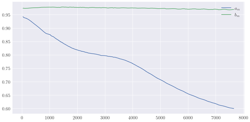
fig, ax = plot_signals(
[
(t_m, a_m, "$a_m$", {}),
(t_m, b_m, "$b_m$", {}),
],
legend="upper right"
)
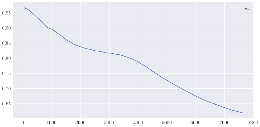
ratio_m = np.divide(a_m, b_m)
fig, ax = plot_signals([(t_m, ratio_m, "$r_m$", {})], legend="upper right")
Degradation Correction (Naive)
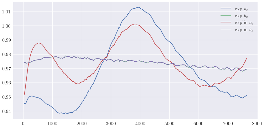
[17]:
from collections import namedtuple
pprint_block("Degradation Correction", level=1)

Correction = namedtuple(
    "Correction",
    [
        "a_m_c",
        "b_m_c",
        "d_a_c",
        "d_b_c",
        "a_c_nn",
        "b_c_nn",
    ]
)
corrections = dict()
for model_name in ["exp", "explin"]:
    degradation_model = load_model(model_name)
    degradation_model.initial_fit(x_a=e_a_m, y_a=a_m, y_b=b_m)

    a_m_c, b_m_c, degradation_model, history = correct_degradation(
        t_m=t_m,
        a_m=a_m,
        e_a_m=e_a_m,
        b_m=b_m,
        e_b_m=e_b_m,
        model=degradation_model,
        verbose=True,
    )

    d_a_c = degradation_model(e_a_nn)
    d_b_c = degradation_model(e_b_nn)
    a_c_nn = np.divide(a_nn, d_a_c)
    b_c_nn = np.divide(b_nn, d_b_c)

    correction = Correction(
        a_m_c, b_m_c, d_a_c, d_b_c, a_c_nn, b_c_nn
    )
    corrections[model_name] = correction

signal_fourplets = []
for model_name in ["exp", "explin"]:
    correction = corrections[model_name]
    signal_fourplets.extend(
        [
            (t_m, correction.a_m_c, "{} $a_c$".format(model_name), {}),
            (t_m, correction.b_m_c, "{} $b_c$".format(model_name), {}),
        ]
    )
_ = plot_signals(signal_fourplets, legend="upper right")


signal_fourplets = []
for model_name in ["exp", "explin"]:
    correction = corrections[model_name]
    signal_fourplets.extend(
        [
            (t_a_nn, correction.d_a_c, "{} $d(e_a(t))$".format(model_name), {}),
            (t_b_nn, correction.d_b_c, "{} $d(e_b(t))$".format(model_name), {}),
        ]
    )
_ = plot_signals(signal_fourplets, legend="lower left")
    Degradation Correction
---------------------------------------------------------------------------
    - Corrected in 3 iterations.
    - Corrected in 3 iterations.

[18]:
# Smoothing and outlier filtering

# Decomposition
c = pywt.wavedec(a_nn, wavelet="db5", mode="per")

# Denoising - Thresholding
thresh = 1.0 * np.nanmax(a_nn)
c[1:] = (pywt.threshold(coeff, value=thresh, mode="soft") for coeff in c[1:])

# Reconstruction
a_nn_r = pywt.waverec(c, wavelet="db5", mode="per")

fig, ax = plot_signals([
    (t_a_nn, a_nn, "$a_{nn}$", {"lw": 2, "alpha": 0.5}),
    (t_a_nn, a_nn_r, "$a_{nn, r}$", {"lw": 1, "c": "k"}),
],
    legend="lower left"
)

[ ]: